Introduction

Create, initialize, and advance a single particle, then optionally export it. The dynamics use only the core installation; the final VTK section requires JaxDEM[io]. The ten-step calculation is deliberately small.

import tempfile
from pathlib import Path

import numpy as np

import jaxdem as jdem

Initialize the Simulation State

First, we create a jaxdem.state.State object. It holds all per-particle data in the simulation. Here we create a single particle at the origin with velocity (1, 0, 0). jaxdem.state.State.create() fills every unspecified attribute with a default value.

state = jdem.State.create(pos=[[0.0, 0.0, 0.0]], vel=[[1.0, 0.0, 0.0]])

Note that we wrote pos=[[coords]], not pos=[coords]. jaxdem.state.State.create() expects a 2-D array of shape (N, dim), so even a single particle needs a list of lists.

Initialize the Simulation System

Next, we create a jaxdem.system.System. It holds the global configuration of the simulation (domain, force model, integrator, …). Like the state, jaxdem.system.System.create() fills in defaults for anything we do not specify. The only requirement is that the system dimension matches the state dimension:

system = jdem.System.create(state.shape, dt=0.01)
state, system = jdem.System.initialize(state, system)

Run the Simulation

After explicit initialization has prepared the initial acceleration, we advance the simulation by calling jaxdem.system.System.step(). Initial forces are prepared by initialize():

n_steps = 10
state, system = system.step(state, system, n=n_steps)
print(f"Advanced {n_steps} steps to time {float(system.time):.3g}")
print("Particle position:", state.pos)
# With no other particle or external force, x(t) = x(0) + v_x * t.
np.testing.assert_allclose(state.pos, [[0.1, 0.0, 0.0]], atol=2e-7)

Advanced 10 steps to time 0.1
Particle position: [[0.09999999 0.         0.        ]]

Saving the Simulation

With the optional [io] extra installed, save the simulation to VTK so we can visualize it in ParaView with VTKWriter. Its save() method writes asynchronously in background threads. Use the writer as a context manager (or call writer.block_until_ready() before exiting) to make sure the writer finishes all files:

tmp_dir = Path(tempfile.mkdtemp(prefix="jaxdem-introduction-"))
try:
    writer = jdem.VTKWriter(directory=tmp_dir)
except ImportError:
    print("Install JaxDEM[io] to run the optional VTK export section.")
else:
    with writer:
        writer.save(state, system)
    print("VTK output for ParaView:", tmp_dir)

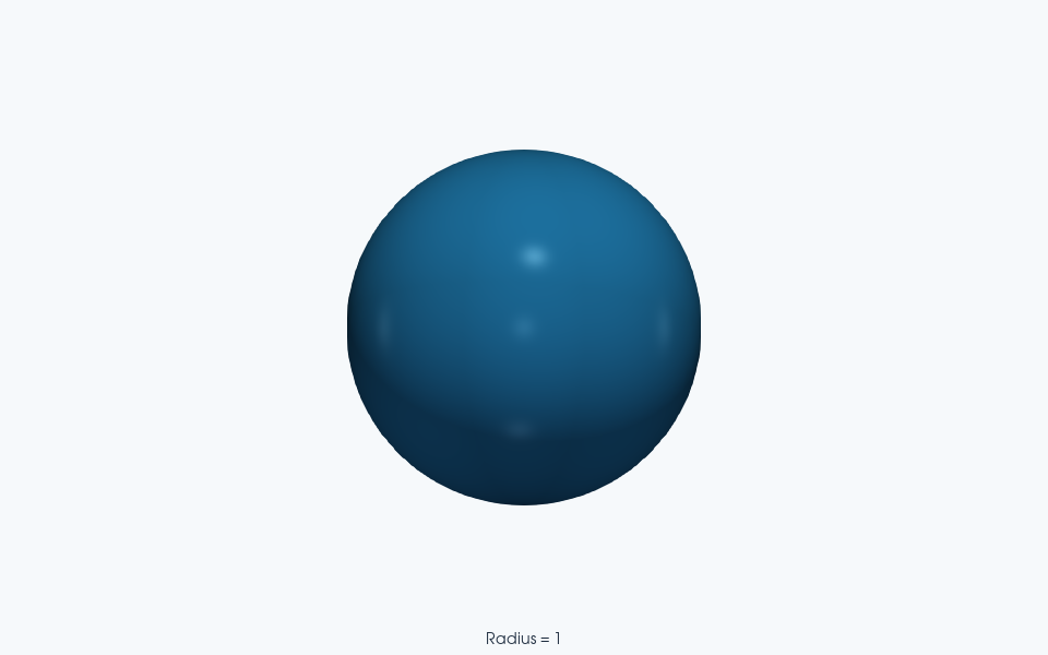
ParaView rendering of this run’s VTKWriter output.

VTK output for ParaView: /tmp/jaxdem-introduction-jzdwvg7p

Where to Go Next

Now that you have seen the simplest simulation, explore the rest of the user guide to learn about each component in depth:

• The Simulation State — particle data, fixed particles, identifiers.

• The Simulation System — system configuration, deactivating modules, batched simulations.

• The Simulation Domain — free, periodic, shear-periodic, and reflective boundaries.

• Integrators and Minimizers — time integration and energy minimization.

• Materials, Matchmakers, and Material Tables — material definitions and matchmakers.

• Force Models — pairwise force laws and species-wise routing.

• The Force Manager — gravity, external forces, custom functions.

• Colliders — contact detection algorithms.

• Clumps (Rigid Bodies) — rigid bodies from multiple spheres.

• Facets (Triangular & Line Boundaries) — flat boundaries from line segments and triangles.

• Deformable Particles — elastic, deformable bodies from bonded meshes.

• VTK Post-Processing and Visualization — exporting frames for ParaView visualization.

• Checkpoint Save and Load — saving and restoring simulations.

• Custom Module Registration and System Usage — registering your own force models, domains, and integrators.