Particle-level friction coefficient of a rigid clump

Same setup as the SASA example, but the quantity of interest is the probe-reported friction coefficient mu = |F_t| / |F_n| instead of the surface area. We take the mean of mu over the sampled approach directions. The directions form a near-uniform Fibonacci lattice on S^2, so the mean is an average over approach solid angle. Equal solid angles generally cover unequal surface areas on a nonspherical body; this is not an area-weighted surface average. The measured force ratio is shape-induced geometric friction, not a material Coulomb coefficient.

The small geometry and probe grids keep this demonstration quick. Increase them separately to check geometric quadrature and directional convergence.

Sphere-ray intersections locate the first contact from outside. Numerics match sasa_calculation.py: x64 resolves the small target_overlap = 1e-10 at the body’s length scale. separation_tolerance = 1e-12 is a compatibility parameter, not an iteration tolerance.

Enable x64 before any other JAX work.

import jax

jax.config.update("jax_enable_x64", True)  # type: ignore[no-untyped-call]

import numpy as np
import matplotlib.pyplot as plt

from jaxdem.utils.particle_creation import create_ga_state, create_sphere_state
from jaxdem.utils.surface_properties import compute_surface_properties

Central rigid clump + tracer sphere

central = create_ga_state(
    N=1,
    nv=8,
    dim=3,
    particle_radius=0.5,
    asperity_radius=0.1,
    particle_type="clump",
    core_type="solid",  # fill the central void so each approach ray meets the body
    n_samples=512,  # modest 3D surface-quadrature budget for a quick demonstration
    seed=0,
    mesh_kwargs={"steps": 50},
)

tracer_radius = 0.05
tracer = create_sphere_state(radii=tracer_radius, dim=3)

Probe the surface

At contact, resolve the net probe force along the center-to-center approach axis \(\hat{\mathbf{d}}\):

\[\mathbf{F}_n=(\mathbf{F}\cdot\hat{\mathbf{d}})\hat{\mathbf{d}},\qquad \mathbf{F}_t=\mathbf{F}-\mathbf{F}_n,\qquad \mu(\hat{\mathbf{d}})= \frac{\lVert\mathbf{F}_t\rVert}{|\mathbf{F}\cdot\hat{\mathbf{d}}|}.\]

Each constituent sphere contact is normal to its own contact surface, but the sum need not point along the two bodies’ COM axis. Roughness therefore produces a tangential resultant without adding a microscopic Coulomb law. On a smooth central sphere the force is radial and this geometric ratio is zero. A vanishing normal resultant makes the ratio singular, so the finite-value check also guards the selected probe setup.

n_points = 128

result = compute_surface_properties(
    central,
    tracer,
    target_overlap=1e-10,
    separation_tolerance=1e-12,
    n_points=n_points,
    n_orientations=1,
    n_rolls=1,
)

mu = np.asarray(result["mu"]).reshape(n_points)
assert np.all(np.isfinite(mu))
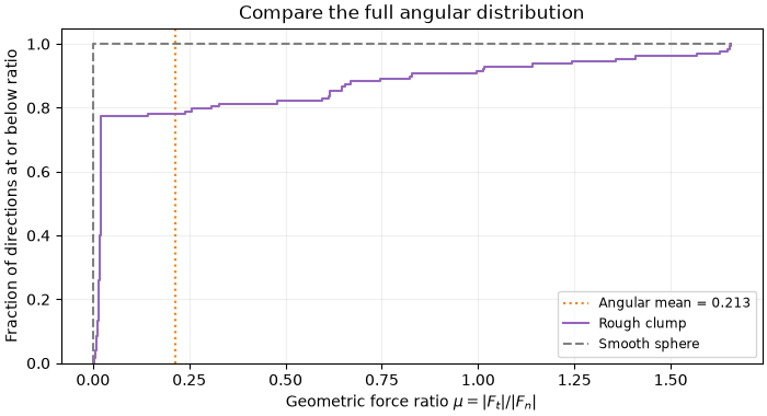
print(f"mu: min={mu.min():.4f}  max={mu.max():.4f}")

mu: min=0.0019  max=1.6554

Mean friction across the sampled approach directions. The Fibonacci lattice approximates the isotropic incident-direction mean

\[\overline{\mu}_{\Omega}=\frac{1}{4\pi} \int_{S^2}\mu(\hat{\mathbf{d}})\,d\Omega \simeq\frac{1}{N_\Omega}\sum_i\mu_i.\]

An area-weighted mean would instead be \(\overline{\mu}_A=\int\mu\,dA/\int dA\). For a radial surface, \(dA/d\Omega=\rho^2\sqrt{1+|\nabla_{S^2}\log\rho|^2}\), so it needs geometric weights absent from the simple arithmetic mean. Choose the averaging measure according to the experiment being represented: an isotropic set of approach directions and uniformly sampled surface area answer different physical questions.

mean_friction = float(mu.mean())
print(f"mean friction = {mean_friction:.4f}")

# A smooth sphere provides a useful baseline: radial normal forces give mu=0.
smooth = create_sphere_state(radii=0.5, dim=3)
baseline = compute_surface_properties(
    smooth,
    tracer,
    target_overlap=1e-10,
    separation_tolerance=1e-12,
    n_points=n_points,
    n_orientations=1,
    n_rolls=1,
)
np.testing.assert_allclose(np.asarray(baseline["mu"]), 0.0, atol=1e-8)
print("Smooth-sphere baseline: mu = 0 within numerical tolerance.")

mean friction = 0.2128
Smooth-sphere baseline: mu = 0 within numerical tolerance.

Examine the distribution behind the mean

Each approach direction has equal weight. The cumulative curve reveals the fraction below any chosen ratio without a bin-width choice. Its difference from the zero-ratio smooth reference comes entirely from shape, since the contact law itself has no tangential friction.

sorted_mu = np.sort(mu)
fractions = np.arange(1, n_points + 1) / n_points
fig, ax = plt.subplots(figsize=(7, 3.8), layout="constrained")
ax.axvline(
    mean_friction,
    color="tab:orange",
    linestyle=":",
    label=f"Angular mean = {mean_friction:.3f}",
)
ax.step(
    np.r_[0.0, sorted_mu],
    np.r_[0.0, fractions],
    where="post",
    color="tab:purple",
    label="Rough clump",
)
ax.plot(
    [0.0, 0.0, sorted_mu[-1]], [0.0, 1.0, 1.0], "--", color="0.5", label="Smooth sphere"
)
ax.set(
    ylabel="Fraction of directions at or below ratio",
    ylim=(0.0, 1.05),
    title="Compare the full angular distribution",
)
ax.legend(fontsize="small")
ax.set_xlabel(r"Geometric force ratio $\mu=|F_t|/|F_n|$")
ax.grid(alpha=0.2)
plt.show()

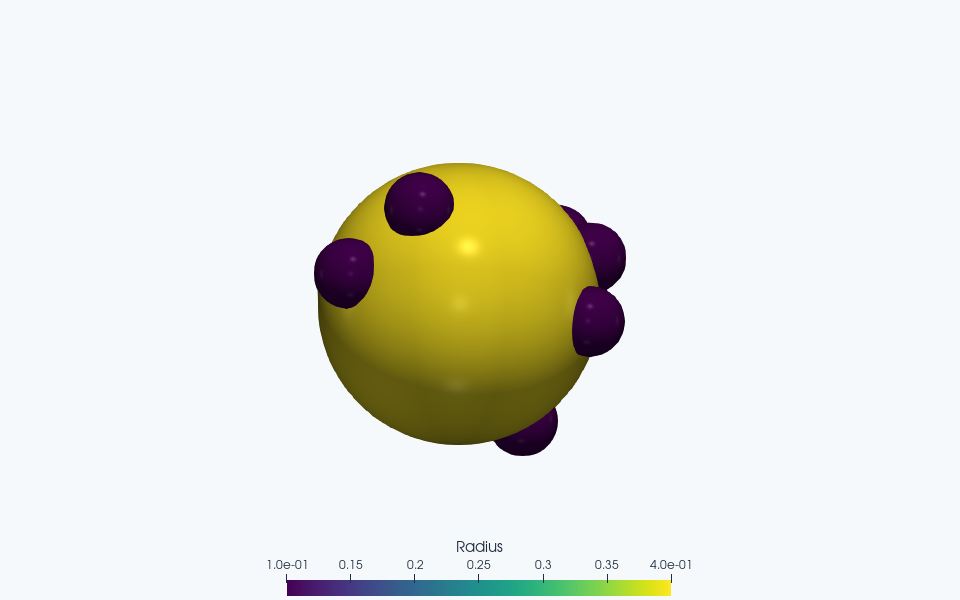
ParaView rendering of this run’s VTKWriter output.